Theory
This section provides an overview of the mathematical formalism underpinning QSWs. The starting point is a discussion of graph theory terminology, which draws primarily from Refs. 1 and 2, followed definition of CTRWs on digraphs and CTQWs on graphs. An overview of the master equation approach to the description of Markovian open systems is then provided. From this, the L-QSW master equation is introduced, which unifies the CTRW and CTQW models under a density theoretic framework. The practical extension of this equation to the inclusion of non-Hermitian absorption and emission process is then presented. Next, the G-QSW is introduced, along with the demoralisation correction scheme. We conclude by discussing vectorization of the QSW master equations, the numerical approximation of which is the primary task at hand.
Digraphs and Graphs
A weighted digraph is defined as a triple \(\mathcal{G} = (V,E,\text{w})\). Vertex set \(V = \{v_1, ...,v_N\}\) is connected by arcs from the set \(E = \{(v_i, v_j), (v_k, v_l),...\}\). Each arc is associated with a positive weight, \(\text{w}(v_i,v_j) \in \mathbb{R}\), which describe the magnitude of connection from \(v_i\) to \(v_j\). \(\mathcal{G}\) is represented by an \(N \times N\) adjacency matrix, \(G\):
Arcs of form \((v_i, v_i)\) are known as self-loops, with a graph containing no self-loops being referred to as a ‘simple graph’. QSW_MPI considers only the case of simple graphs, as such \(\text{Tr}(G) = 0\).
Associated with \(\mathcal{G}\) is the weighted but undirected graph \(\mathcal{G}^u = (V,E^u,\text{w}^u)\), where \(E^u\) is a set of edges associated with weights \(\text{w}^u\). This is represented by a symmetric adjacency matrix, \(G^u\), with \(\text{w}^u(v_i,v_j)= \text{max}(\text{w}(v_i,v_j),\text{w}(v_j,v_i))\) according to Equation (1). A digraph is weakly connected if there exists a path between all \(v_i \in \mathcal{G}^u\). Additionally, a digraph which satisfies the further condition of having a path between all \(v_i \in \mathcal{G}\) is strongly connected.
The number of arcs (or edges) incident on vertex \(v_j\),
is termed the vertex degree and the total sum of the incident edge weights on vertex \(v_j\),
is termed the weighted vertex in-degree. Similarly, the total sum of the outgoing edge weights at vertex \(v_i\),
is termed the weighted vertex out-degree. A vertex, \(v_i\), with \(\text{OutDeg}(v_i) > 0\) and \(\text{InDeg}(v_i) = 0\) is refered to as a source. Conversely, a vertex, \(v_j\), with \(\text{InDeg}(v_j) > 0\) and \(\text{OutDeg}(v_j) = 0\) is refered to as a sink. A graph with constant \(\text{Deg}(v_i)\), or a digraph satisfying the additional condition of \(\text{OutDeg}(v_i) = \text{InDeg}(v_i)\) for all \(v_i \in \mathcal{G}\), is referred to as a regular graph.
Continuous-Time Classical Random Walks
A continuous-time random walk (CTRW) describes the probabilistic evolution of a system (walker) though a parameter space as a continuous function of time. Most typically, CTRWs refer to a type of Markov process. This describes a scenario where the future state of a system depends only on its current state. Heuristically, one might describe such systems as having ‘no memory’. Under this condition, a CTRW over a digraph is described by a system of first-order ordinary differential equations,
where element \(p_i \geq 0\) of \(\vec{p}(t)\) is the probability of the walker being found at \(v_i\), and \(\vec{p}(t)\) has the solution \(\vec{p}(t) = \exp(-tM)\vec{p}(0)\) which satisfies \(\sum\vec{p}(t) = 1\)3,4. \(M\) is the transition matrix derived from \(G\),
where the off-diagonal elements \(M_{ij}\) represent the probability flow along an edge from \(v_j\) to \(v_i\), while the diagonal elements \(M_{jj}\) account for the total outflow from \(v_j\) per unit time. Scalar \(\gamma \in \mathbb{R}\) is the system wide transition rate2.
Continuous-Time Quantum Walks
A continuous-time quantum walk (CTQW) is constructed by mapping \(\mathcal{G}\) to an \(N\)-dimensional Hilbert space where the set of its vertices \(\{\lvert v_1 \rangle, ..., \lvert v_N \rangle\}\) form an orthonormal basis. The matrix elements of the system Hamiltonian \(H\) are then equal to the classical transition matrix (\(\langle v_j \rvert H\lvert v_i \rangle = M_{ij}\)). In place of \(\vec{p}(t)\), the evolution of the state vector \(\lvert \Psi(t) \rangle = \sum_{i=1}^{N} \lvert v_i \rangle\langle v_i \vert \Psi(t) \rangle\) is considered, the dynamics of which are governed by the Schrödinger equation2,
which has the formal solution \(\lvert \Psi(t) \rangle = \exp(-\frac{i}{\hbar}tH)\lvert \Psi(0) \rangle\) when \(H\) is time-independent. The probability associated with vertex \(v_i\) at time \(t\) is \(|\langle v_i \vert \Psi(t) \rangle|^2\).
While Equations (4) and (6) appear superficially similar, there are several fundamental differences between the two processes. Firstly, \(\lvert \Psi(t) \rangle\) describes a complex probability amplitude, meaning that its possible paths may interfere. Secondly, the Hermiticity requirement on \(H\) needed to maintain unitary evolution of the system dictates that \(M\) be derived from \(\mathcal{G}^u\)4.
Markovian Open Quantum Systems
A density matrix,
describes a statistical ensemble of quantum states, \(\lvert \Psi_k(t) \rangle\), each with an associated probability \(p_k \geq 0\) and \(\sum_k p_k = 1\). The case where \(p_k\) is non-zero for more than one \(k\) is termed a ‘mixed’ state while the case of only one non-zero \(p_k\) is termed a ‘pure’ state. The dynamics of \(\rho(t)\) are given by the Liouville-von Neumann equation,
which is the density theoretic equivalent of the Schrödinger equation (Equation (6))5. In a quantum walk context, entries \(\rho_{ii}\) (termed ‘populations’) represent the probability density at a given vertex while off-diagonal elements \(\rho_{ij}\) describe phase coherence between vertices \(v_i\) and \(v_j\)2.
Consider a system, \(S\), coupled to an external reservoir (or ‘bath’), \(B\). The Hilbert space of \(S + B\) is given by5,
where \(\mathcal{H}_S\) and \(\mathcal{H}_B\) are the Hilbert spaces of \(S\) and \(B\). \(S\) is referred to as an ‘open’ system, while \(S + B\) is closed in the sense that its dynamics can be described unitarily. Under the condition that the evolution of \(S\) is Markovian with no correlation between \(S\) and \(B\) at t = 0, and given \(\mathcal{H}_S\) of finite dimensions \(N\). The dynamics of \(S\) are described by a generalization of Equation (8): the GKSL quantum master equation5,
with
where \(H\) is the Hamiltonian describing the unitary dynamics of \(\mathcal{H}_s\), the Lindblad operators, \(L_k\), span the Liouville space and scalars \(\tau_k \geq 0\). The reduced density operator \(\rho_s(t)\) is formed by tracing out the degrees of freedom associated with \(B\). Equation (10) is invariant under unitary transformations of the Lindblad operators, allowing for the construction of a wide range of phenomenological models.
Quantum Stochastic Walks
Local Environment Interaction
A local-interaction quantum stochastic walk (L-QSW) on an arbitrary simple \(\mathcal{G}\) is derived from Equation (11) by defining \(\rho_s(t)\) in the basis of vertex states, \(\{\lvert v_1 \rangle,...,\lvert v_N \rangle\}\), setting \(H\) equal to the transition matrix of \(G^u\), and deriving the local interaction Lindblad operators from the transition matrix of \(G\),
where \(k=N(j-1)+i\). Each \(L_k\) describes an incoherent scattering channel along an arc of \(\mathcal{G}\) when \(i \neq j\) and dephasing at \(v_i\) when \(i = j\)2,4.
A scalar decoherence parameter \(0 \leq \omega \leq 1\) is introduced4. This allows for the model to be easily tuned to explore a continuum of mixed quantum and classical dynamics. The standard form of a QSW is then,
with \(\rho_s(t)\) denoted as \(\rho(t)\) and \(\tau_k = 1\) for all dissipator terms. At \(\omega = 0\), Equation (13) reduces to a CTQW obeying the Liouville-von Neumann equation (Equation (8)) and, at \(\omega = 1\), the density-matrix equivalent of the CTRW equation (Equation (4)) is obtained.
It is worth noting that QSWs are defined elsewhere directly from \(G\) and \(G^u\), such that \(\langle v_j \rvert L_k\lvert v_i \rangle = G_{ij}\) and \(\langle v_j \rvert H\lvert v_i \rangle = G^u_{ij}\)6. Additionally, the continuous-time open quantum walk (CTOQW) 7 defines quantum walks on undirected graphs obeying Equation (10), where \(H\) is defined by Equation (5) and, in place of \(\sqrt{M_{ij}}\) in Equation (12), is the canonical Markov chain transition matrix,
In each case, these walks are consistent with the generalised definition of QSWs with locally-interacting Lindblad operators4.
For L-QSWs, a predictable block structure in \(\tilde{\mathcal{L}}\) means that the L-QSW super-operator can be efficiently constructed directly from the CSR representations of \(H\) and a single-matrix representation of the local-interaction Lindblad operators,
thus avoiding the need to form intermediate Kronecker products or store each Lindblad operator separately.
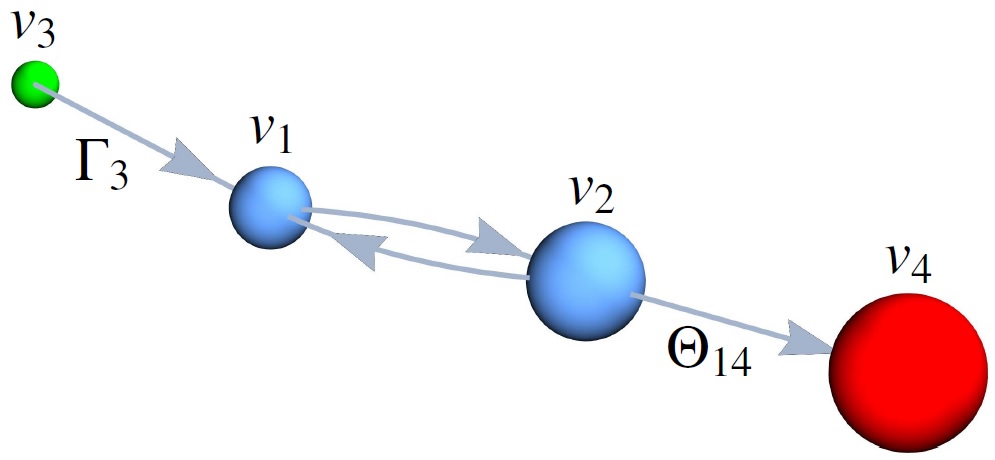
Fig. 1 A dimer graph with a source, \(v_3\), attached to \(v_1\) with absorption rate \(\Gamma_{3}\) and sink, \(v_4\) attached to \(v_2\) with emission rate \(\Theta_{14} = 3\) (see Equations (16)) and ((17)).
The local interaction QSW model naturally facilitates the modelling of non-Hermitian transport through connected \(\mathcal{G}\). This is achieved by introducing a source vertex set, \(V^\Gamma\), and a sink vertex set, \(V^\Theta\), which are connected unidirectionaly to \(\mathcal{G}\) by arc sets \(E^\Gamma\) and \(E^\Theta\). Together with \(\mathcal{G}\), these form the augmented digraph, \(\mathcal{G}^{\text{aug}}\). For example, consider the dimer graph shown in Fig. 1 on which absorption is modeled at \(v_1\) and emission at \(v_2\). In QSW_MPI, \(G^u\) and \(G^{\text{aug}} = G + G^\Gamma + G^\Theta\) are represented as,
The walk Hamiltonian is then derived from \(G^u\) and the \(L_k\) corresponding to scattering and dephasing on \(\mathcal{G}\) from \(G\). Finally, \(L_k\) originating from \(\mathcal{G}^\Gamma\) and \(\mathcal{G}^\Theta\) are formed as \(\langle v_j \rvert L_k\lvert v_i \rangle = G^{\Gamma}_{ij}\) and \(\langle v_j \rvert L_k\lvert v_i \rangle = G^{\Theta}_{ij}\) respectively, appearing in additional terms appended to Equation (13) outside the scope of \(\omega\). An L-QSW incorporating both absorptive and emissive processes is then succinctly expressed as,
where \(k = \tilde{N}(j-1) + i\) with \(\tilde{N}\) equal to \(N\) plus the total vertices in \(V^\Gamma\) and \(V^\Theta\), and \(\rho(t)\) is of dimensions \(\tilde{N} \times \tilde{N}\). Terms \(\mathcal{D}^{\Gamma}_k[\rho(t)]\) are defined as per Equation (11) with \(\tau_k = \Gamma_k\) where \(\Gamma_k\) is the absorption rate from source \(v_j \in \mathcal{G}^\Gamma\) to vertex \(v_i \in \mathcal{G}\). Similarly, for \(\mathcal{D}^{\Theta}_k[\rho(t)]\), \(\tau_k = \Theta_k\) where \(\Theta_k\) is the emission rate from vertex \(v_j \in \mathcal{G}\) to sink \(v_i \in \mathcal{G}^{\Theta}\).
Global Environment Interaction
A global-interaction quantum stochastic walk (G-QSW) differs from an L-QSW in that it utilizes a single Lindblad operator derived from the digraph adjacency matrix,
However, a Lindblad operator of this form has the potentially undesirable effect of inducing transitions between not-connected vertices with outgoing arcs incident on a common vertex, a phenomena termed spontaneous moralisation. A demoralisation correction scheme can be applied to arrive at a non-moralising G-QSW (NM-G-QSW), which respects the connectivity of the originating digraph. This proceeds by a homomorphic mapping of \(\mathcal{G}\) and \(\mathcal{G}^u\) to an expanded vertex space1. First supported by QSWalk.jl6, provided here is a practical overview of the process which is implemented in QSW_MPI with respect to weighted digraphs.
Graph Demoralisation
From \(\mathcal{G}^u = (V, E^u, \text{w}^u)\), construct a set of vertex subspaces \(V^D = \{V^D_i\}\) with,
\[\begin{split}V^D_i = \begin{cases} \{v^0_i,...,v^{\text{Deg}(v_i)-1}_i\}, & \text{Deg}(v_i)>0 \\ \{v^0_i\}, & \text{Deg}(v_i) = 0 \end{cases}\end{split}\]for each \(v_i \in V\). Associated with \(V^D\) is edge set \(E^{uD} = \{(v^i_j,v^k_l), (v^m_n,v^o_p),...\}\), where \((v^l_i,v^k_j) \in E^{uD} \iff (v_i,v_k) \in E^u\). These have weights,
(19)¶\[ \text{w}^{uD}(V_i^D,V_k^D) = \left(\text{SubDeg}(V_i^D,V_k^D)\text{w}^u(v_i,v_k)\right)^{-\frac{1}{2}}\]where \(\text{SubDeg}(V^D_i,V^D_k) = \dim(\{(v_i^l,v_k^j) : (v_i^l,v_k^j) \in E^{uD}\})\). This forms the demoralised graph, \(\mathcal{G}^{uD} = (V^D,E^{uD}, \text{w}^{uD})\).
Construct the demoralised digraph, \(\mathcal{G}^D = (V^D,E^D,\text{w}^D)\) where \((v_i^j,v_k^l) \in E^D \iff (v_i,v_k) \in E\). Arc weights, \(\text{w}^D(V^D_i,V^D_k)\), are given by Equation (19) with \(\text{w}(v_i,v_k)\) in place of \(\text{w}^u(v_i,v_k)\) and \(E^D\) in place of \(E^{uD}\).
Form the Lindblad operator from orthogonal matrices, \(\{F_i\}\in \mathbb{C}^{\dim(V^D_i) \times \dim(V^D_i)}\), such that,
(20)¶\[ L^D = [F_i]_{j+1,k}\text{G}^{D}_{v_i^j,v_k^l}\lvert v^j_i \rangle \langle v^l_k \rvert,\]and QSW_MPI follows the convention of choosing for \(\{F_i\}\) the Fourier matrices6.
Construct the rotating Hamiltonian,
(21)¶\[\begin{split} \langle v^k_l \rvert H^D_{\text{rot}} \lvert v^i_j \rangle = \begin{cases} \text{i}, & l=j \text{ and } i = k + 1 \\ -\text{i}, & l=j \text{ and } i = k - 1 \\ 0, & \text{otherwise} \end{cases}\end{split}\]which changes the state within subspaces of \(V^D\) in order to prevent occurrence of stationary states dependant only on the expanded vertex set of \(\mathcal{G}^D\).
Through formation of \(L^D\), spontaneous moralisation is destroyed but its induced dynamics may not correspond with symmetries present in \(\mathcal{G}\). In this case, symmetry may be reintroduced by constructing additional \(L^D\) using unique permutations of \(\{F_i\}\). However, the generality of this symmetrisation process has not been confirmed1. The master equation of a NM-G-QSW is then,
where \(H^D\) is formed from \(\mathcal{G}^{uD}\) as per Equation (5). The probabilities of the demoralised density operator, \(\rho^{D}(t)\), are related to the probability of measuring the state in vertex \(v_i\) at time \(t\) by
Vectorization of the Master Equation
Equations (13), (17) and (22) may be recast as a system of first order differential equations through their representation in an \(\tilde{N}^2 \times \tilde{N}^2\) Liouville space5, where \(\tilde{N}\) is the dimension of the system. This process, termed ‘vectorization’, makes use of the identity \(\text{vec}(XYZ) = (Z^T \otimes X)\text{vec}(Y)\)8 to obtain the mappings,
where \(X, Y, Z \in \mathbb{C}^{\tilde{N} \times \tilde{N}}\). Such that, for each QSW variant, its equation of motion has the solution,
where the vectorized density operator, \(\tilde{\rho}(t)\), is related \(\rho(t)\) by \(\tilde{\rho}(t)_k = \rho(t)_{ij}\) with \(k = \tilde{N}(j-1) + i\).
For an L-QSW on \(\mathcal{G}\) (Equation (13)),
is the vectorized superoperator. The vectorized forms of \(\tilde{\mathcal{L}}\) for Equations (17) and (22) are trivially obtained by comparison to Equations (13) and (26).
Package Overview
QSW simulation occurs through use of the
MPI submodule which allows the creation of distributed
\(\tilde{\mathcal{L}}\), vectorization of \(\rho(0)\), and
evolution of the system dynamics. In particular, the user creates and
calls methods from one of the following walk classes:
LQSW: L-QSWs (Equations (13) and (17)).GQSW: G-QSWs (Equation (18) and (22)).GKSL: Walks obeying the GKSL master equation (Equation (10)).
A walk object is instantiated by passing to it the relevant
operators, coefficients and MPI-communicator. On doing so the
distributed \(\tilde{\mathcal{L}}\) is generated and its 1-norm
series calculated [1]. After this the user defines \(\rho(0)\) and
generates the distributed \(\tilde{\rho}(0)\) via the
initial_state() method.
Simulations are carried out for a single time point with the step()
method or for a number of equally spaced points using the series()
method. These return \(\tilde{\rho}(t)\) (or
\(\tilde{\vec{\rho}}(t)\)) as a distributed vectorized matrix(s)
which can be reshaped and gathered to a specified MPI process via
gather_result(), or measured via gather_populations(). Otherwise,
results may be reshaped and saved directly to disk using save_result()
or save_population(). File I/O is carried out using h5py10, a
Python interface to the HDF5 libraries, and will default to MPI
parallel-I/O methods contained in the non-user accessible
parallel_io` module if such operations are supported by the
host system. Finally, a second user accessible module
operators provides for creation of L-QSW and NM-G-QSW
operators from \(\mathcal{G}\) stored in the SciPy CSR matrix
format11.
The following provides an overview of QSW_MPI workflows using examples drawn from prior studies. These correspond to files included in ‘examples’ folder of the QSW_MPI package. In addition to the program dependencies of QSW_MPI, the example programs make use of the Python packages Networkx12 for graph generation, and Matplotlib13 for visualisation. Note that a complete accounting of the methods contained in QSW_MPI exceeds the scope of this document. Comprehensive documentation and installation instructions are included with the package and are additionally hosted on Read the Docs14.
Usage Examples
Execution
QSW_MPI programs, and other Python 3 programs utilising MPI, are executed with the command,
mpirun -N <n> Python3 <program_file.py>
where <n> is a user-specified parameter equal to the number of MPI
processes.
Graph Demoralisation
Here we provide an example of the typical workflow of QSW_MPI through an exploration of the graph demoralisation process. This begins by loading the required modules and external methods.
import qsw_mpi as qsw
import numpy as np
from scipy.sparse import csr_matrix as csr
from mpi4py import MPI
As the system explored in this example is small, its simulation will not
benefit from multiple MPI processes. However, initialisation of an MPI
communicator is required to use the MPI module.
comm = MPI.COMM_WORLD
Adjacency matrices \(G\) and \(G^u\) are defined here by writing
them directly into the CSR format, where the arguments of csr are an
ordered array of non-zero values, a corresponding tuple containing the
row indices and column indices, and the dimensions of the adjacency
matrix. The structure of the directed graph and its undirected
counterpart is shown in :numref::digraph and Fig. 3.
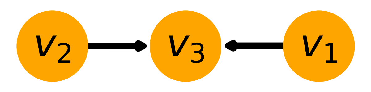
Fig. 2 Example digraph. |
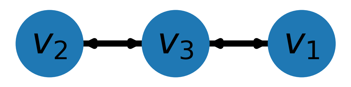
Fig. 3 Example graph. |
G = csr(([1,1],([2,2],[0,1])),(3,3))
GU = csr(([1,1,1,1],([0,1,2,2],[2,2,0,1])),(3,3))
First, we examine the behaviour of a G-QSW. The Lindblad operator and Hamiltonian are created as per Equations (5) and (18). Note that the Lindblad operator is contained within an array.
gamma = 1.0
Ls = [G]
H = qsw.operators.trans(gamma, GU)
Next, the starting state of the system is specified as a pure state at \(v_1\). This may be achieved by either specifying \(\rho(0)\) completely or by giving a list of probabilities, in which case its off-diagonal entries are assumed to be \(0\). Here, the latter approach is employed.
rho_0 = np.array([1,0,0])
A GQSW() walk object is now initialised with \(\omega = 1\), such
that the dynamics induced by \(L_{\text{global}}\) can be examined
in isolation. The initial state of the system is then passed to the walk
object.
omega = 1.0
GQSW = qsw.MPI.GQSW(omega, H, Ls, comm)
GQSW.initial_state(rho_0)
Using the step() method the state of the system at \(t = 100\) is
examined. Note that the result is gathered to a single MPI process. As
such, commands acting on the gathered array should be contained within a
conditional statement which first checks for the correct MPI process
rank.
GQSW.step(t = 100)
rhot = GQSW.gather_result(root = 0)

if comm.Get_rank() == 0:
    print(np.real(rhot.diagonal()))
After the period of evolution, we find that there is a non-zero probability of there being a walker at \(v_2\), despite it having a degree of 0.
>> [0.25 0.25 0.5]
This is an example of spontaneous moralisation, a non-zero transition probability between \(v_1\) and \(v_3\) occurs due to them having a common ‘child’ node.
We will now demonstrate how to use QSW_MPI to apply the demoralisation correction scheme. First, we create a set of vertex subspaces, \(V^D\).
vsets = qsw.operators.nm_vsets(GU)
These are then used with adjacency matrices G and GU to create the Hamiltonian, Lindblad operators and rotating Hamiltonian which capture the structure of the demoralised graph and demoralised digraph.
H_nm = qsw.operators.nm_H(gamma, GU,vsets)
L_nm = [qsw.operators.nm_L(gamma, G,vsets)]
H_loc = qsw.operators.nm_H_loc(vsets)
When creating the GQSW walk object, it is initialised with
additional arguments specifying the vertex subspaces and rotating
Hamiltonian.
nm_GQSW = qsw.MPI.QSWG(omega, H_nm, L_nm,
                       comm, H_loc = H_loc,
                       vsets = vsets)
The initial system state is then mapped to the moralised graph as per Equation (23),
rho_0_nm = qsw.operators.nm_rho_map(rho_0, vsets)
and passed to the walk object via initial_state(). System
propagation and measurement proceeds as previously described. At
\(t = 100\) the system is now in a pure state at the sink node, as
expected by the originating graph topology.
>> [3.72007598e-44 0.00000000 1.00000000]
As a further point of consideration, we will now compare the dynamics of
the NM-G-QSW to an L-QSW on the same digraph, with \(H\) and
\(M_L\) defined as the adjacency matrices GU and G. Note
that \(M_L\) is provided as a single CSR matrix.
LQSW = qsw.MPI.LQSW(omega, GU, G, comm)
LQSW.initial_state(rho_0)
Evolving the state to \(\rho(100)\) with step() yields,
>> [-9.52705648e-18 0.00000000 1.00000000]
which corresponds to the state of the NM-G-QSW.
The coherent evolution of the two systems is examined by first rebuilding \(\tilde{\mathcal{L}}\) at \(\omega = 0\).
GQSW.set_omega(0)
LQSW.set_omega(0)
After which a step() to \(t = 100\) yields,
>> [3.80773381e-07 9.98766244e-01 1.23337485e-03]
for the NM-G-QSW and,
>> [3.80773217e-07 9.98766244e-01 1.23337485e-03]
for the L-QSW. In fact, for this particular system, the limiting
dynamics of a NM-G-QSW correspond to that of a CTQW and CTRW, as is the
case for the L-QSW. However, if we examine the time evolution of the two
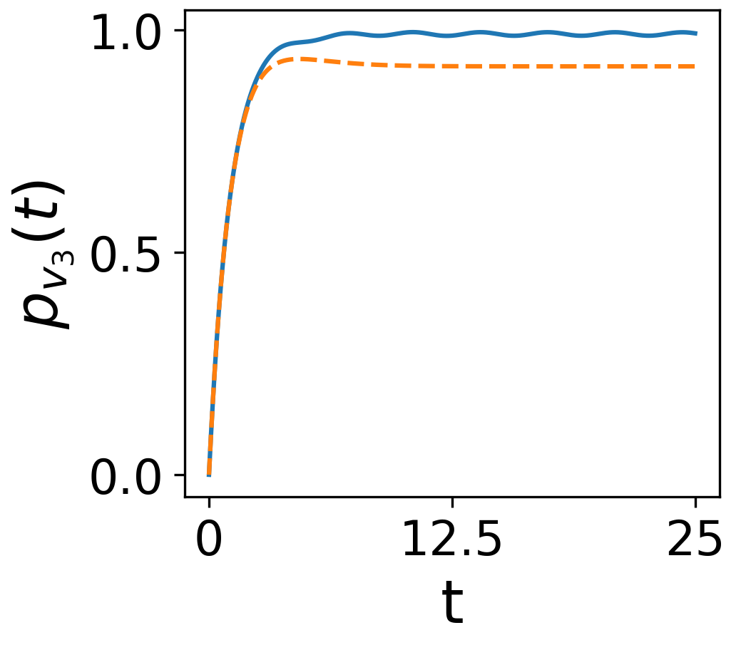
systems at \(\omega = 0.9\) using the series() method,
nm_GQSW.series(t1=0,tq=25,steps=500)
LQSW.series(t1=0,tq=25,steps=500)
notably different dynamics are observed. As shown in Fig. 4, the NM-G-QSW results in a higher transfer of probability to the sink vertex and does not as readily decay to a quasi-stationary state.
Graph Dependant Coherence
Here the steady-state solutions for an L-QSW on a full binary tree graph
and a cycle graph are examined with respect to support for coherence.
The graphs were generated and converted to sparse adjacency matrices
using NetworkX and L-QSWs defined as per Equation
(13) using the LQSW subclass.

Fig. 5 2-branching tree-graph. |
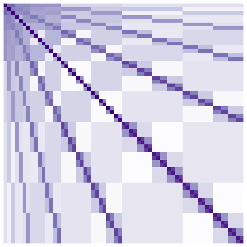
Fig. 6 \(|\rho(t_{\infty})|\). |
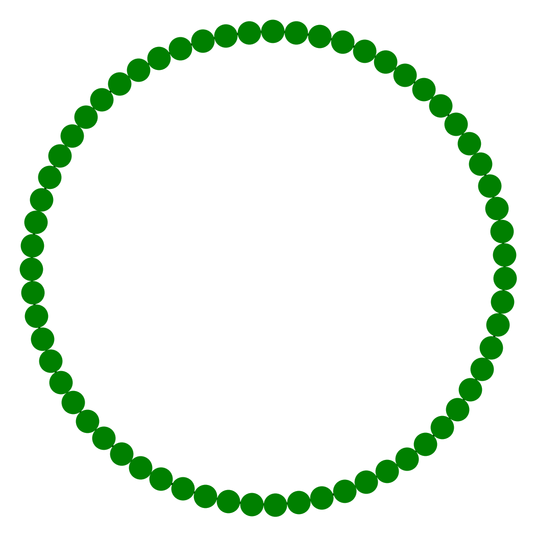
Fig. 7 60 vertex cycle graph. |
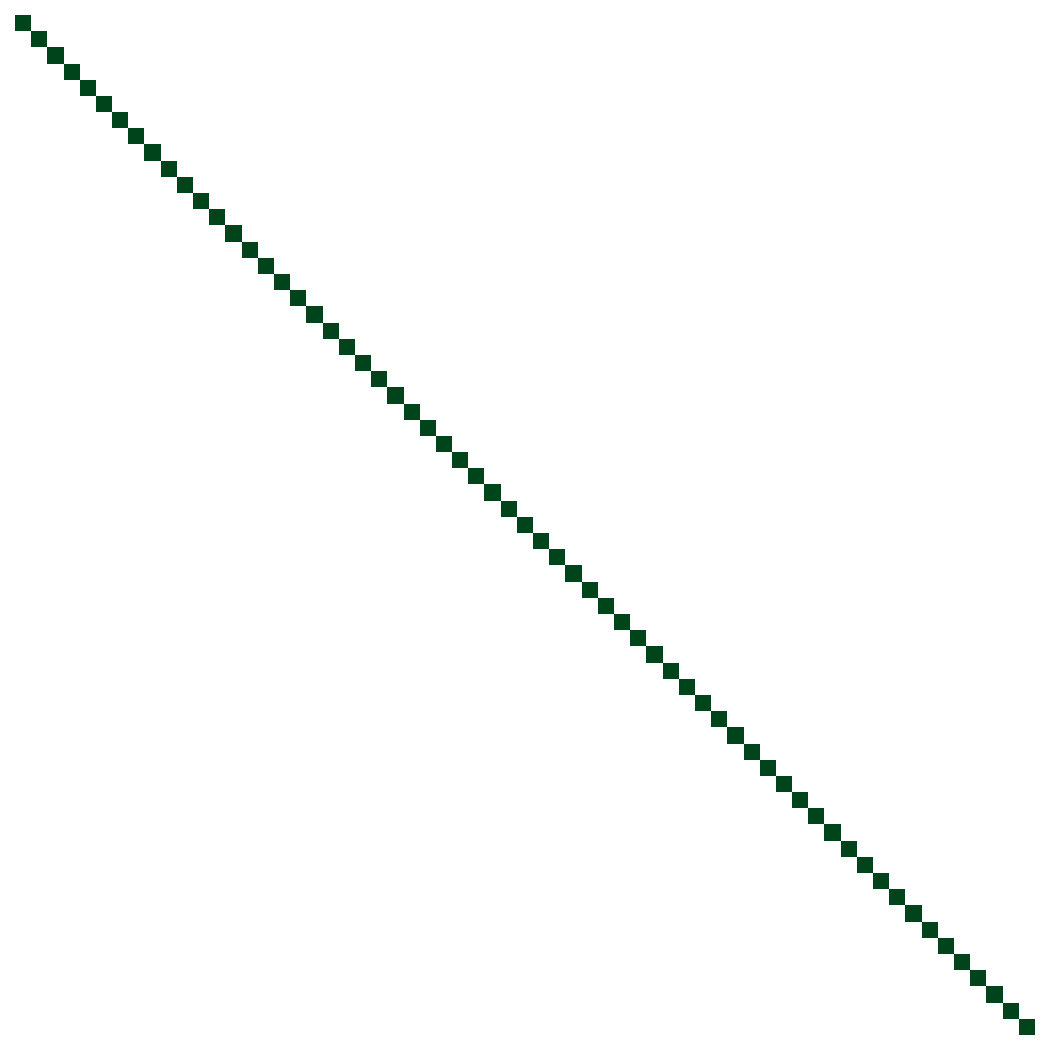
Fig. 8 \(|\rho(t_{\infty})|\). |
Starting in a maximally mixed state, \(\rho(0)\), was evolved via
the step() method to the steady-state, \(\rho(\infty)\), by
choosing a sufficiently large time (\(t = 100\)). This is visualised
in Fig. 5, Fig. 6, Fig. 7 and Fig. 8,
where it is apparent that \(\rho(\infty)\) for the balanced tree exhibits significant
coherence, as opposed to the cycle graph which exhibits none. In fact,
it has been established that \(\rho(\infty)\) for regular graphs
will always exhibit no coherence7.
Transport Through a Disordered Network
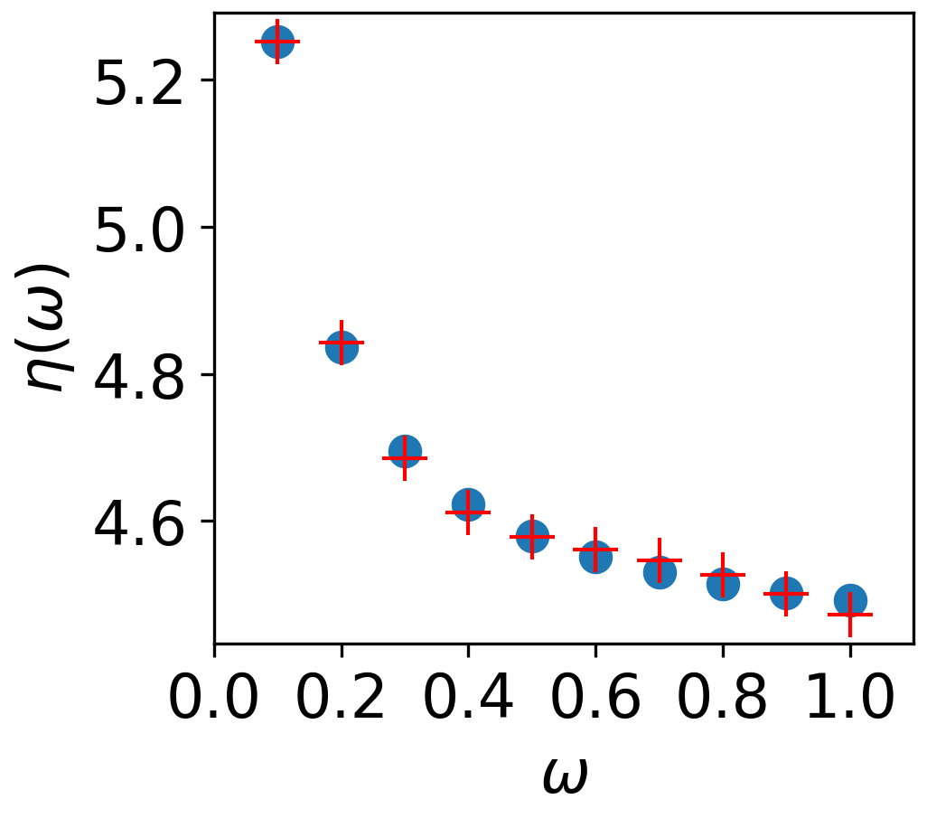
Fig. 9 Expected survival time of the network and optimised dimer (\(\delta = 1.5\)) after 43 evaluations of the objective function. Starting parameters of the dimer were \(V =\Gamma_D = \gamma_d = 0.5\).
This example makes use of time series calculations to illustrate that the efficiency of transport through a disordered network, as modelled by an L-QSW, can be closely approximated as transport through an energetically disordered dimer15. A system of \(N\) points randomly distributed in a unit sphere undergoing dipole-dipole interactions is considered, leading to the potential,
which is set equal to \(G\). A source with \(\Gamma = 0.5\) is attached to \(v_1\) and a sink with \(\gamma = 0.5\) to \(v_N\).
The efficiency of transport is quantified through the Expected Survival Time (EST),
where \(p_\gamma\) is the accumulated population at the sink vertex.
Numerically this is approximated by making use of the series() method
to calculate \(1 - p_\gamma(t)\) at \(q\) evenly spaced
intervals between \(t_1 = 0\) and some time \(t_q\) where
\(p_\gamma(t) \approx 1\). The resulting vector is then numerically
integrated using the Simpson’s Rule method provided by SciPy. By
repeating this for a series of omega values where
\(0 < \omega \leq 1\), the response of \(\eta(\omega)\) is
specified for the network.
An energetically disordered dimer is described by the Hamiltonian,
where \(V\) represents the hopping rates between the vertices and \(\delta\) is the energetic disorder. To this, a source of rate \(\Gamma_D\) is attached to the first vertex and a sink of rate \(\gamma_D\) to the second. The response of \(\eta(\omega)\) between \(0 < \omega \leq 1\) is then determined as previously described.
To arrive at values of \(V\), \(\Gamma_D\) and \(\gamma_D\)
which produce a similar \(\eta(\omega)\) response, the problem is
formulated as an optimisation task with the objective function being
minimisation of the difference in EST between the disordered network and
dimer at corresponding \(\omega\) values. For this, the SciPy
least_squares optimisation algorithm was used. The result of the
fitting process is shown in Figure
Fig. 9 for a network with
\(N = 10\). Despite being a much simpler system, the dimer closely
approximates \(\eta(\omega)\) of the disordered network.
References
1 K. Domino, A. Glos, and M. Ostaszewski, Quantum Information and Computation 17, (n.d.).
2 P.E. Falloon, J. Rodriguez, and J.B. Wang, Computer Physics Communications 217, 162 (2017).
3 N.G. Kampen, Stochastic Processes in Physics and Chemistry (Elsevier, 2007).
4 J.D. Whitfield, C.A. Rodríguez-Rosario, and A. Aspuru-Guzik, Physical Review A 81, (2010).
5 H.-P. Breuer and F. Petruccione, The Theory of Open Quantum Systems, Nachdr. (Clarendon Press, Oxford, 2009).
6 A. Glos, J.A. Miszczak, and M. Ostaszewski, Computer Physics Communications 235, 414 (2019).
7 C. Liu and R. Balu, Quantum Information Processing 16, 173 (2017).
8 S. Banerjee and A. Roy, Linear Algebra and Matrix Analysis for Statistics (CRC Press, 2014).
9 A. Al-Mohy and N. Higham, SIAM Journal on Scientific Computing 33, 488 (2011).
10 A. Collette, Python and Hdf5: Unlocking Scientific Data (“O’Reilly Media, Inc.”, 2013).
11 E. Jones, T. Oliphant, and P. Peterson, (2001).
12 A.A. Hagberg, D.A. Schult, and P.J. Swart, in Proceedings of the 7th Python in Science Conference, edited by G. Varoquaux, T. Vaught, and J. Millman (Pasadena, CA USA, 2008), pp. 11–15.
13 J.D. Hunter, Computing in Science & Engineering 9, 90 (2007).
14 E. Matwiejew, (2020).
15 P. Schijven, J. Kohlberger, A. Blumen, and O. Mülken, Journal of Physics A: Mathematical and Theoretical 45, 215003 (2012).
| [1] | Selection of optimal series expansion terms, \(m\), and scaling and squaring parameter, \(s\), is achieved through backwards error analysis dependant on \(A_{\text{norms}} = \{||A^n||_1\}\), where \(n = 1,...,9\) and \(||.||_1\) is the matrix 1-norm9. As \(||tA^n||_1 = t ||A^n||\), \(A_\text{norms}\) is reusable for all exponentiations at the same \(\omega\). It is thus included as part of the \(\tilde{\mathcal{L}}\) construction phase. |